Fast Fourier transform
Fourier transforms are useful
Can we calculate them efficiently?
The discrete Fourier transform
Change of basis in a finite dimensional space
Maps signal sampled at \(N\) regularly spaced time points to representation at \(N\) frequency points \[ F_n = \sum_{j=0}^{N-1} f_j e^{-i\eta_n j},\qquad \eta_n\equiv \frac{2\pi n}{N} \]
\(F_n\) contain same information as \(f_j\), and \(f_j\) can be recovered completely by inverting operation
Note that \(e^{-i\eta_n j}=e^{-i\eta_{n-N} j}\) so we can extend definition \(F_n=F_{N-n}\)
- Key to inverting \[ \sum_{n=0}^{N-1} e^{i\eta_n j} = \begin{cases} 0 & j\neq 0 \mod N\\ N & j = 0 \mod N. \end{cases} \]
One way to show this is via \[ z^N-1 = (z-1)(1 + z + z^2 +\cdots z^{N-1}) \] Can you fill in the argument? Note: \(e^{i\eta_n}\) are \(N\)th roots of 1
Inverting gives \[ f_j = \frac{1}{N}\sum_{n=0}^{N-1} F_n e^{i\eta_n j}. \]
“Democratic” definition would have \(1/\sqrt{N}\) in both definitions
DFT then change of basis to orthonormal basis \(e^{(n)}_j = \frac{e^{i\eta_n j}}{\sqrt{N}}\)
Both DFT and its inverse then unitary
Fourier transforms with complex exponentials have positive and negative frequencies
Here \(\eta_n\) values for \(n\) close to \(N-1\) are the negative frequencies since \(e^{-i\eta_n j}=e^{2\pi ij -i\eta_n j}=e^{i\eta_{N - n}j}\)
Several limits to consider…
\(N\to\infty\) limit
\(\eta_n\) values become dense in range \((-\pi,\pi]\), with separation \(\Delta \eta = 2\pi/N\)
Replace sum in IDFT integral according to: \[ \sum_{n=0}^{N-1} \left(\cdots\right) \xrightarrow{N\to\infty} N \int_{0}^{2\pi} \frac{d\eta}{2\pi}\left(\cdots\right) \] \[ f_j = \int_{0}^{2\pi} \frac{d\eta}{2\pi}\,F(\eta) e^{i\eta j} \]
\(N\to\infty\) with \(f_j = f(jL/N)\)
\(N\to\infty\) limit samples \(f(x)\) ever more finely in range (0,L]
Now DFT becomes an integral \[ \hat f(k) \equiv \int_0^L f(x) e^{-ik_n x}\,dx, \] where \(k_n =2\pi n/L\). Note that \(k_n x = \eta_n j\). \[ \begin{align} \hat f_k &= \int_0^L f(x) e^{-ik_n x}\,dx\nonumber\\ f(x) &= \frac{1}{L}\sum_k \hat f_k e^{ik_n x} \end{align} \]
\[ \begin{align} \hat f_k &= \int_0^L f(x) e^{-ik_n x}\,dx\nonumber\\ f(x) &= \frac{1}{L}\sum_k \hat f_k e^{ik_n x} \end{align} \]
- Now \(\hat f_k\) has extra dimension of distance (on account of integral), which gets removed by the \(1/L\) in inverse \[ \frac{1}{L}\sum_k e^{ik x} = \delta_L(x) \] \(\delta_L(x)\) is an \(L\)-periodic version of the \(\delta\)-function.
\(L\to\infty\)
- Finally Fourier transform, where we take \(L\to\infty\), so that inverse transform becomes an integral too \[ \begin{align} \hat{f}(k) & = \int_{-\infty}^\infty f(x) e^{-ik_n x}\,dx\nonumber\\ f(x) &= \int_{-\infty}^\infty \hat f(k) e^{ik_n x}\,\frac{dk}{2\pi} \label{coll_FTTrans} \end{align} \]
Some important properties
- Some properties of DFT (and all of the above)
If \(f_j\) is real then \(F_n = \left[F_{-n}\right]^*\).
If \(f_j\) is even (odd), \(F_n\) is even (odd).
(Ergo) if \(f_j\) is real and even, so is \(F_n\).
Higher dimensions
Generalizes to higher dimensions straightforwardly
If data lives \(d\) dimensions with \(N_i\) datapoints along dimension \(i=1,\dots d\) \[ F_{\mathbf{n}} = \sum_{\mathbf{n}} f_\mathbf{j}e^{-i \boldsymbol{\eta}_\mathbf{n}\cdot \mathbf{j}} \] \(\mathbf{j}=(j_1,\ldots j_{d})\) with \(j_i = 0,\ldots N_i - 1\) and \(\boldsymbol{\eta}_\mathbf{n} = 2\pi (n_1 / N_1, \ldots n_d/ N_d)\) \(n_i = 0,\ldots N_i - 1\)
Fast Fourier transform
\[ F_n = \sum_{j=0}^{N-1} f_j e^{-i\eta_n j} \]
What is complexity of computing the Fourier transform?
DFT is matrix-vector multiplication \[ \mathbf{F} = Q \cdot \mathbf{f}. \] where matrix has elements \(Q_{n j}\equiv e^{-i\eta_n j}\)
Naively, complexity is \(O(N^2)\)
Can do a lot better than this, because of structure of \(Q\)!
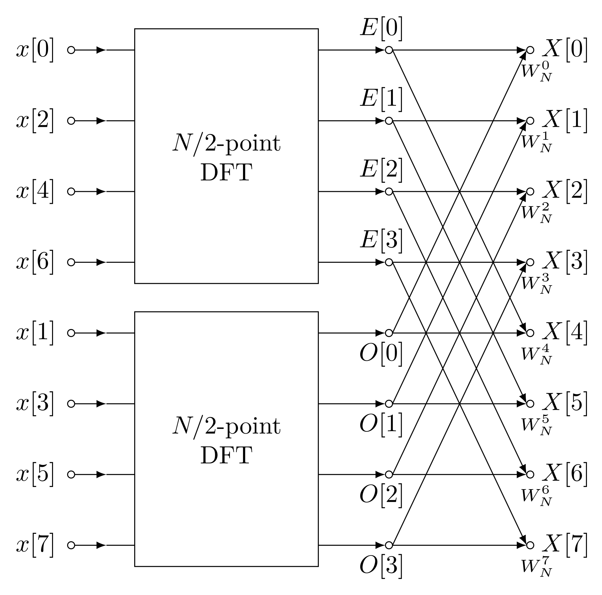
Divide and conquer pattern: break problem up into two sub-problems
\[ f^{\text{e}}_j = f_{2j}\qquad f^{\text{o}}_j = f_{2j+1},\qquad j=0,\ldots N/2 - 1. \]
- Key idea: we are going to express DFT \(F_n\) in terms of DFT of \(f^\text{e}_j\) and \(f^\text{o}_j\)
- Write \(\omega_N \equiv e^{2\pi i/N}\), so that \(e^{i\eta_n j}=\omega_N^{nj}\) and DFT is
\[ F_n = \sum_{j=0}^{N-1} f_j \omega_N^{-nj} \] \[ \begin{align} F_n &= \sum_{j=0}^{N-1} \omega_N^{-nj} f_j \\ &=\sum_{j=0}^{N/2-1} \left[\omega_N^{-2nj} f^{\text{e}}_j + \omega_N^{-n(2j+1)}f^{\text{o}}_j\right]\\ &=\sum_{j=0}^{N/2-1} \left[\omega_{N/2}^{-nj} f^{\text{e}}_j + \omega_N^{-n}\omega_{N/2}^{-nj}f^{\text{o}}_j\right] \end{align} \]
\[ F_n =\sum_{j=0}^{N/2-1} \left[\omega_{N/2}^{-nj} f^{\text{e}}_j + \omega_N^{-n}\omega_{N/2}^{-nj}f^{\text{o}}_j\right] \]
Already looking like sum of two DFTs of size \(N/2\)
Write \(n\) as \[ n = (N/2)n_0 + n' \] where \(n_0=0,1\) and \(n'=0,\ldots N/2 - 1\).
If \(n\) a power of 2, \(n_0\) is most significant bit of \(n\) when written in binary and \(n'\) are remaining bits
\[ n = (N/2)n_0 + n' \]
- Since \(\omega_{N/2}^{-jn}=\omega_{N/2}^{-jn'}\) we have
\[ \begin{align} F_n &= \sum_{j=0}^{N/2-1} \left[\omega_{N/2}^{-nj} f^{\text{e}}_j + \omega_N^{-n}\omega_{N/2}^{-nj}f^{\text{o}}_j\right]\\ &=\sum_{j=0}^{N/2-1} \left[\omega_{N/2}^{-n'j} f^{\text{e}}_j + (-1)^{n_0}\omega_N^{-n'} \omega_{N/2}^{-n'j}f^{\text{o}}_j\right]\\ &= F^\text{e}_{n'} + (-1)^{n_0}\omega_N^{-n'} F^\text{o}_{n'} \end{align} \]
\[ F_n = F^\text{e}_{n'} + (-1)^{n_0}\omega_N^{-n'} F^\text{o}_{n'} \]
- If \(N\) a power of 2 can repeat process until we get length 1
Complexity
Clear that FFT is going to beat the naive approach
\(T(N)\) is steps required to compute DFT for size \(N\) input
Calculating \(F^\text{e}_{n'}\) and \(F^\text{0}_{n'}\) takes time \(2T(N/2)\)
Combining to evaluate \(F_n\) is a further \(N\) steps, so
\[ T(N) = 2T(N/2) +\Theta(N) \]
- This implies \(T(N)=\Theta(N\log N)\)
What if \(N\) isn’t a power of 2?
Use divide and conquer strategy for any other factor \(p\) of \(N\)
If largest prime factor of \(N\) is bounded i.e. doesn’t grow with \(N\) this still yields \(T(N)=\Theta(N\log N)\)
If \(N\) is prime you have to use something else
Best to ensure \(N\) is a power of two e.g. by choosing size of simulation appropriately or padding data with zeros
History
Modern invention of FFT is credited to Cooley and Tukey (1965). First to discuss complexity
Divide and conquer approach anticipated in radio astronomy by David Wheeler in Cambridge (see Ryle (1975)) and Danielson and Lanczos (1942), for applications in crystallography
OG is Carl Friedrich Gauss in 1805 (predating even Fourier) in his astronomical studies
See Cooley, Lewis, and Welch (1967) for more on historical background
FFT in Python
Several helper functions available to make your life easier:
np.fft.fftfreq(n, d), which returns the frequencies (not the angular frequencies) for input size \(n\) and sample spacing \(d\).np.fft.fftshift(A)shifts data so that the zero frequency is in the centre.np.fft.ifftshift(A)inverts this.
Simple example
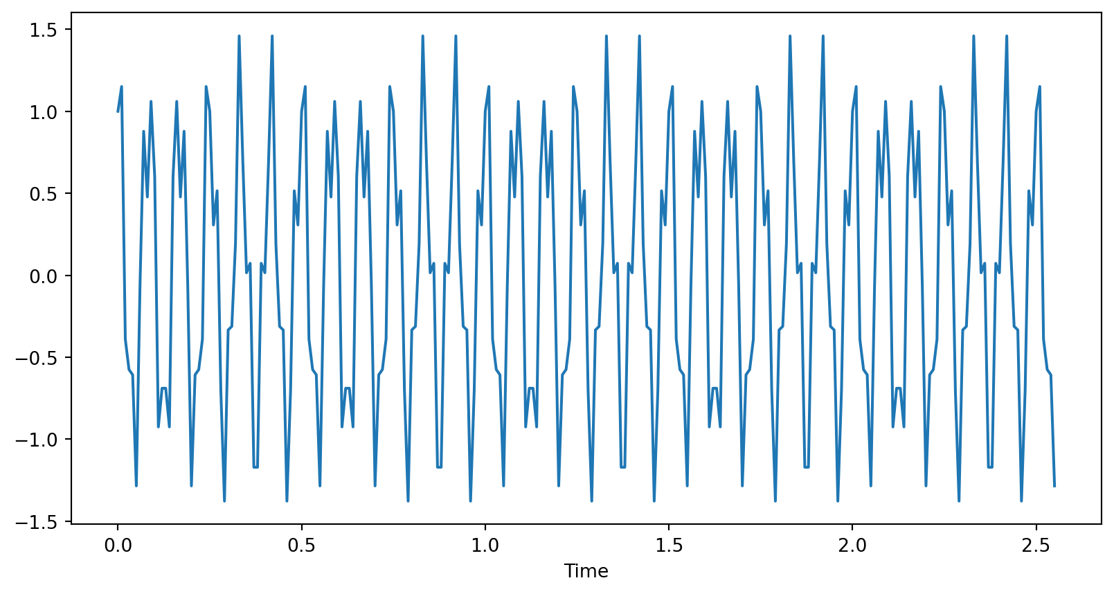
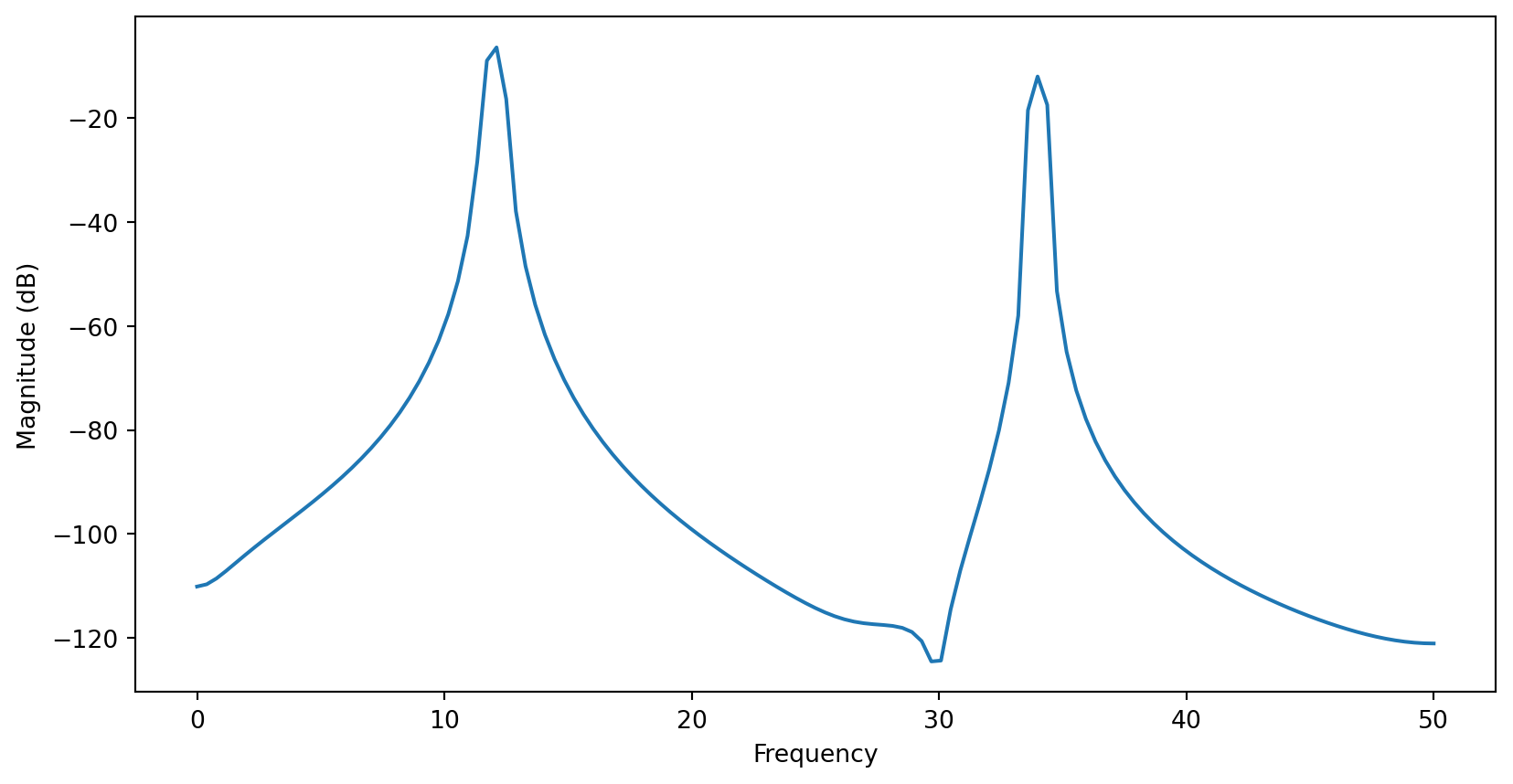
- Signal consisting of two sinusoids at 12 Hz and 34 Hz:
- Take FFT and plot vs array index
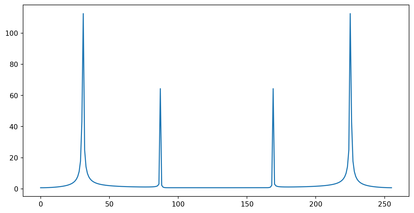
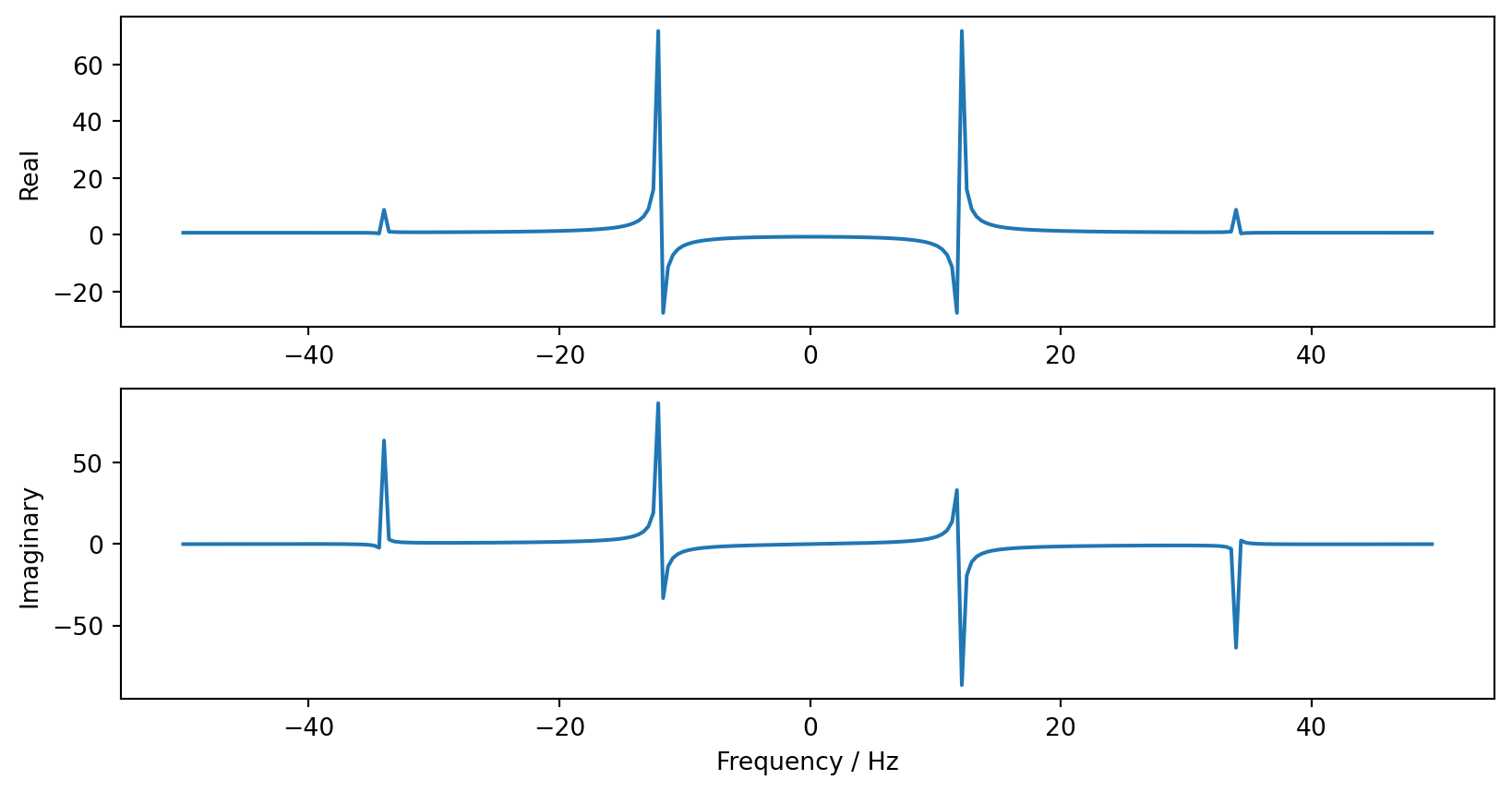
- Or against real frequency (sample spacing of \(dt=0.01\))

- Fourier transform of real valued data has property \(F_n = \left[F_{-n}\right]^*\):
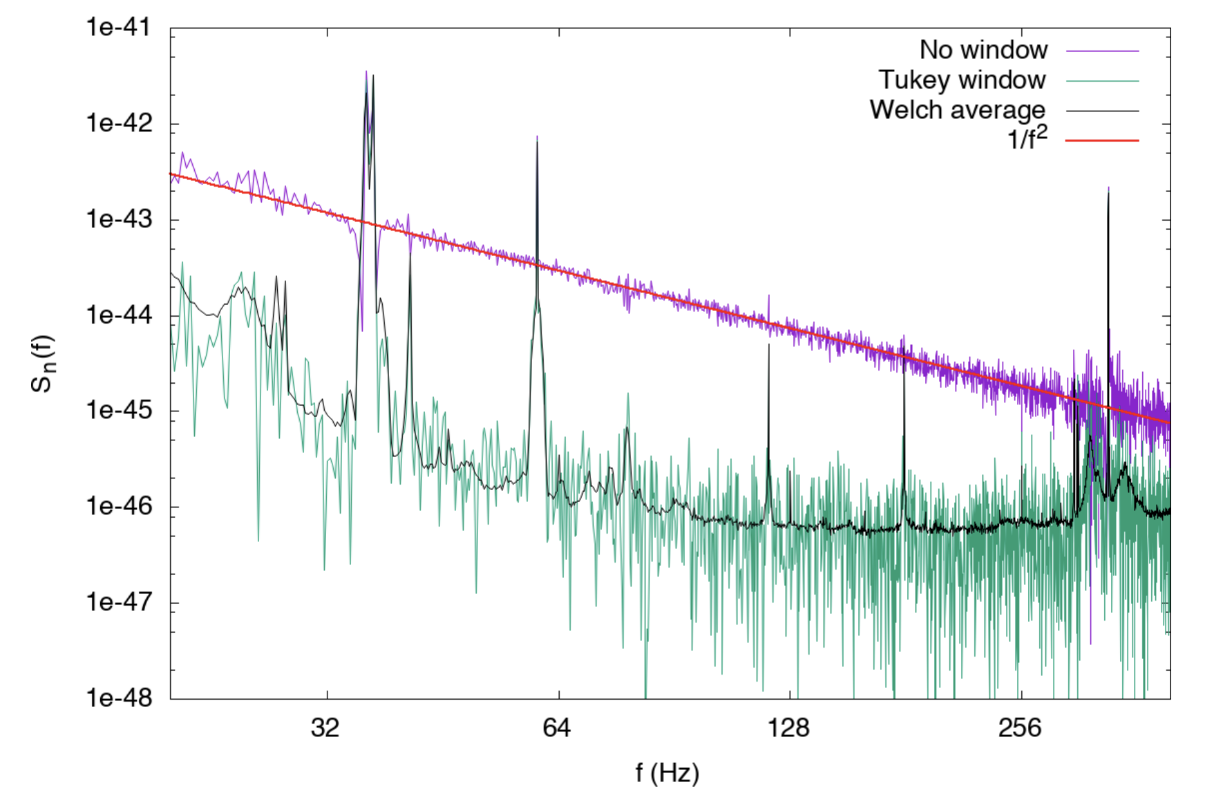
Windowing
- Signal a pair of sinusoids, but FFT not just \(\delta\)-functions
- Because data is of finite length
Windowing causes FFT to be non-zero outside the frequencies present in the signal: spectral leakage
Sharp window means that FFT is effectively convolved with FT of top hat i.e. a sinc function
If window happens to contain a whole number of wavelengths of the signals present, spectral leakage does not occur
Chose different window functions e.g. with smooth edges
Rectangular / top hat window has low dynamic range: bad at distinguishing contributions of different amplitude even when their frequencies differ
Leakage from large peak may obscure smaller ones
It has high resolution: good at resolving peaks of similar amplitude that are close in frequency
Usually several options (Hamming, Tukey (him again), etc.) when using library functions that perform spectral analysis
Applications of FFT
Mindboggling number of applications from signal processing in experimental data, audio and video signals, to numerical simulation
We’ll look at two examples…
Signal processing
Time series data from LIGO and Virgo experiments on gravitational wave detection that led to the 2017 Nobel prize in physics
See Abbott et al. (2020) for details, as well as accompanying notebook that describes how analysis is performed in Python
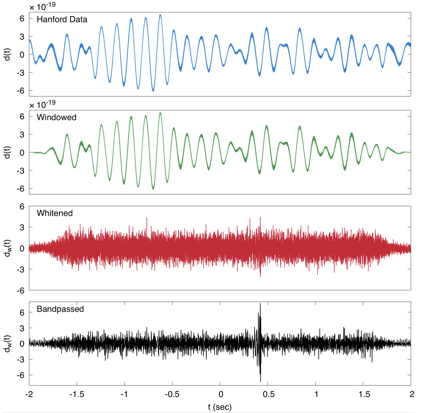
Uncovering the signal in the raw data involves a number of processing steps designed to eliminate noise, mostly carried out in Fourier domain
Guiding principle is that the noise is stationary — described by a random process that does not change in time — while signal is transient
This idea can be used to reduce noise in the data even though low frequency noise completely dominates the raw measurement (top panel)
First step is windowing to reduce spectral leakage
Next, data is whitened: Fourier spectrum is normalized by spectral density \[ \tilde d(f)\longrightarrow \frac{\tilde d(f)}{S_n^{1/2}(f)} \]
Idea is to prevent high amplitude noise in certain parts of the spectrum from swamping the signal
After this step (third panel, red trace), the low frequency noise has been greatly reduced
Finally, filter with a pass band [35 Hz, 350 Hz], removing low frequency seismic noise and high frequency (quantum) noise from detector
Filtering is Fourier analog of windowing
At this point, a transient is revealed in the data (bottom panel)
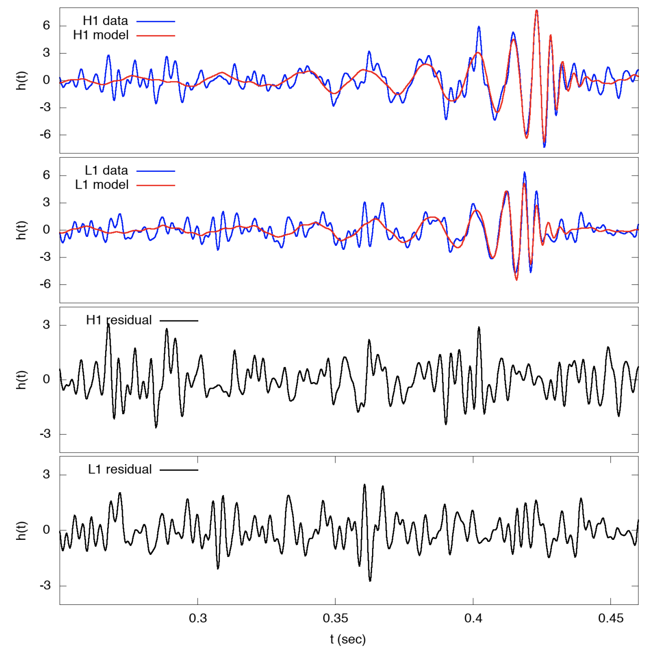
Fit transient with a model that describes graviational wave physics
Important check is to analyze residual — difference between data and model — and to check whether it is described by a stationary noise process
The phases of Fourier components should be random and uncorrelated, for example
Partial differential equations
Spectral methods exploit FFT as part of solver
Example: time-dependent Schrödinger equation
\[ i\hbar \frac{\partial \psi}{\partial t} = -\frac{\hbar^2}{2m}\nabla^2 \psi + V(\mathbf{r})\psi \]
When potential is absent, solutions are superpositions of plane waves
\[ \Psi_\mathbf{k}(\mathbf{r}, t) = \exp\left[-i\frac{\hbar^2 \mathbf{k}^2 t}{2m} +i\mathbf{k}\cdot\mathbf{r}\right] \tag{1}\]
- If KE absent, evolution would be
\[ \Psi(\mathbf{r}, t) = \Psi(\mathbf{r}, 0)\exp\left[-iV(\mathbf{r})t/\hbar\right] \tag{2}\]
Idea behind split-step method is that time evolution can be approximated by alternating Equation 1 and Equation 2
Equation 1 requires that we express the solution in terms of plane wave components… FFT!
- Write equation in operator form as
\[ i\hbar \frac{\partial \ket{\psi}}{\partial t} = H\ket{\psi} = (T+V)\ket{\psi} \]
Solution is \(\ket{\psi(t)} = \exp(-iHt/\hbar)\ket{\psi}(0)\)
Exponential of \(A+B\) obeys Lie product formula
\[ e^{A+B} = \lim_{n\to\infty}\left( e^{A/n}e^{B/n}\right)^n. \]
More precisely, \[ e^{xA}e^{xB} = e^{x(A+B) + O(x^2)}. \]
More accurate approximation is Suzuki—Trotter formula
\[ e^{xA/2}e^{xB}e^{xA/2} = e^{x(A+B) + O(x^3)} \]
- Here’s a simple 1D example:
def split_step_schrodinger(psi_0, dx, dt, V, N, x_0 = 0., k_0 = None, m = 1.0, non_linear = False):

    len_x = psi_0.shape[0]

    x = x_0 + dx*np.arange(len_x)

    dk_x = (2*np.pi)/(len_x*dx)
    if k_0 == None:
        k_0 = -np.pi/dx
    k_x = k_0+dk_x*np.arange(len_x)

    psi_x = np.zeros((len_x,N), dtype = np.complex128)
    psi_k = np.zeros((len_x,N), dtype = np.complex128)
    psi_mod_x = np.zeros((len_x), dtype = np.complex128)
    psi_mod_k = np.zeros((len_x), dtype = np.complex128)
    psi_x[:,0] = psi_0

    if not non_linear:
        V_n = V(x)
    else:
        V_n = V(x,psi_0)

    def _compute_psi_mod(j):
        return (dx/np.sqrt(2*np.pi))*psi_x[:,j]*np.exp(-1.0j*k_x[0]*x)

    def _compute_psi(j):
        psi_x[:,j] = (np.sqrt(2*np.pi)/dx)*psi_mod_x*np.exp(1.0j*k_x[0]*x)
        psi_k[:,j] = psi_mod_k*np.exp(-1.0j*x[0]*dk_x*np.arange(len_x))

    def _x_half_step(j,ft = True):
        if ft == True:
            psi_mod_x[:] = np.fft.ifft(psi_mod_k[:])
        if non_linear:
            V_n[:] = V(x,psi_x[:,j])
        psi_mod_x[:] = psi_mod_x[:]*np.exp(-1.0j*(dt/2.)*V_n)

    def _k_full_step():
        psi_mod_k[:] = np.fft.fft(psi_mod_x[:])
        psi_mod_k[:] = psi_mod_k[:]*np.exp(-1.0j*k_x**2*dt/(2.*m))

    def _main_loop():
        psi_mod_x[:] = _compute_psi_mod(0)

        for i in range(N-1):
            _x_half_step(i,ft = False)
            _k_full_step()
            _x_half_step(i)
            _compute_psi(i+1)

    _main_loop()

    return psi_x,psi_k,k_x
Abbott, Benjamin P, Rich Abbott, Thomas D Abbott, Sheelu Abraham, Fausto Acernese, Kendall Ackley, Carl Adams, et al. 2020. “A Guide to LIGO–Virgo Detector Noise and Extraction of Transient Gravitational-Wave Signals.” Classical and Quantum Gravity 37 (5): 055002.
Cooley, James W, Peter AW Lewis, and Peter D Welch. 1967. “Historical Notes on the Fast Fourier Transform.” Proceedings of the IEEE 55 (10): 1675–77.
Cooley, James W, and John W Tukey. 1965. “An Algorithm for the Machine Calculation of Complex Fourier Series.” Mathematics of Computation 19 (90): 297–301.
Danielson, Gordon Charles, and Cornelius Lanczos. 1942. “Some Improvements in Practical Fourier Analysis and Their Application to x-Ray Scattering from Liquids.” Journal of the Franklin Institute 233 (5): 435–52.
Ryle, Martin. 1975. “Radio Telescopes of Large Resolving Power.” Science 188 (4193): 1071–79.