Linear algebra

Numerical linear algebra is a huge topic
We’ll look at how common operations are performed in NumPy and SciPy, and some applications in physics

Linear algebra with NumPy

Multiplying matrices is easy in NumPy using np.matmul
@ operator gives shortcut

import numpy as np
A = np.random.rand(3, 3)
B = np.random.rand(3, 3)
np.matmul(A, B), A @ B

(array([[0.64405657, 0.71384765, 0.29837612],
        [1.18686062, 1.33454843, 0.59619047],
        [1.6478261 , 1.57803648, 0.85193837]]),
 array([[0.64405657, 0.71384765, 0.29837612],
        [1.18686062, 1.33454843, 0.59619047],
        [1.6478261 , 1.57803648, 0.85193837]]))

You’ll get an error if your matrices don’t match…

C = np.random.rand(2, 3)
D = np.random.rand(4, 2)
C @ D

ValueError: matmul: Input operand 1 has a mismatch in its core dimension 0, with gufunc signature (n?,k),(k,m?)->(n?,m?) (size 4 is different from 3)

If either A or B has rank greater than two: treat as a stack of matrices, with each matrix in last two indices
Usual broadcasting rules then apply to remaining indices

C = np.random.rand(4, 3, 3)
D = np.random.rand(3, 3)
(C @ D).shape

(4, 3, 3)

Several library functions to perform matrix and vector algebra, including
- np.dot (dot product)
- np.vdot (dot product including complex conjugation)
- np.trace, etc.

Most versatile is np.einsum: explicitly translate expressions using the Einstein summation convention

\[ \left[A\cdot B\right]_{ik} = \sum_{j} A_{ij}B_{jk} = A_{ij}B_{jk} \]

np.einsum('ij,jk->ik', A, B)

array([[0.64405657, 0.71384765, 0.29837612],
       [1.18686062, 1.33454843, 0.59619047],
       [1.6478261 , 1.57803648, 0.85193837]])

\[ \operatorname{tr}\left[A\cdot B\right] = \sum_{i,j} A_{ij}B_{ji} = A_{ij}B_{ji} \]

np.einsum('ij,ji->', A, B)

2.830543378941007

In what order should multiple contractions be evaluated?
How should loops be nested?
Recall: should evaluate $M_1 M_2\cdots M_n \mathbf{v}$ as $O(N^2)$ matrix-vector multiplications, rather than $O(N^3)$ matrix-matrix multiplications followed by matrix-vector multiplication
In general no efficient algorithm to find best way!
einsum can use a “greedy” algorithm (contracting pair of tensors with lowest cost at each step)
Information on contraction order provided by np.einsum_path

Inversion (np.linalg.inv)
Calculation of determinant (np.linalg.det)
Eigenvalues and eigenvectors (np.linalg.eig or np.linalg.eigh for hermitian problems)

…inherit their complexity from $O(N^3)$ complexity of matrix multiplication

Power method

Better methods available if only want largest (or smallest) eigenvalue and eigenvector (e.g. QM ground state)
Simplest is Power method
- Start from arbitrary vector $\mathbf{b}_0$
- Multiply repeatedly by matrix $A$
- Result tends to dominant eigenvector (largest magnitude eigenvalue)

Convenient to normalize each time

\[ \mathbf{b}_{k+1} = \frac{A \mathbf{b}_k}{\lVert A\mathbf{b}_k\rVert} \]

\[ \lim_{k\to\infty}\mathbf{b}_k = \mathbf{v}_\text{dom} \]

\[ A\mathbf{v}_\text{dom} = \lambda_\text{dom}\mathbf{v}_\text{dom} \]

Already met this idea when we discussed Markov chains
Relevant matrix was $\mathsf{P}_{jk}=p(j|k)\geq 0$ of transition probabilities, which is stochastic:

\[ \sum_j \mathsf{P}_{jk} = 1 \]

Guarantees that dominant eigenvalue is one and dominant eigenvector has interpretation of the stationary distribution

PageRank

Google’s PageRank algorithm assesses relative importance of webpages based on structure of links between them

PageRank imagines a web crawler navigating between pages according to a transition matrix $\mathsf{P}$
Stationary distribution $\boldsymbol{\pi}$ satisfying\[ \mathsf{P}\boldsymbol{\pi} = \boldsymbol{\pi} \] then interpreted as a ranking
Page $j$ more important than page $k$ if $\boldsymbol{\pi}_j>\boldsymbol{\pi}_k$

Problem if Markov chain is non-ergodic: state space breaks up into several independent components, leading to nonunique $\boldsymbol{\pi}$

\[ \begin{equation} \mathsf{P}=\begin{pmatrix} 0 & 1 & 0 & 0 \\ 1 & 0 & 0 & 0 \\ 0 & 0 & 0 & 1 \\ 0 & 0 & 1 & 0 \end{pmatrix} \end{equation} \]

First two pages and last two do not link to each other, so $\boldsymbol{\pi}^T = \begin{pmatrix} \pi_1 & \pi_1 & \pi_2 & \pi_2 \end{pmatrix}$ is a stationary state for any $\pi_{1,2}$

Way out is to modify Markov chain to restore ergodicity and give a unique $\boldsymbol{\pi}$
Crawler either moves as before with probability $\alpha$ or moves with probability $1-\alpha$ to a random webpage \[ \alpha\mathsf{P} + (1-\alpha)\mathbf{t} \mathbf{e}^T \] where $\mathbf{e}^T= (1, 1, \ldots 1)$ and $\mathbf{t}$ is a “teleporting” vector
Matrix has positive (i.e. $>0$) entries: there is a unique stationary state (and hence ranking)
Further modification is required to teleport away from “dangling” webpages without any outgoing links

Power method is basis of more sophisticated algorithms such as Lanczos iteration
All based on idea that matrix-vector products preferred over matrix-matrix products
Provide only incomplete information about eigenvalues and eigenvectors

Sparsity

Many matrices that we meet in physical applications are sparse, meaning that most of elements are zero

\[ \left[-\frac{\hbar^2}{2m}\frac{d^2}{dx^2} + V(x)\right]\psi(x) = E\psi(x) \]

\[ \frac{d^2}{dx^2} \sim \frac{1}{\Delta x^2}\begin{pmatrix} -2 & 1 & 0 & 0 & 0 & \cdots & 1 \\ 1 & -2 & 1 & 0 & 0 & \cdots & 0 \\ 0 & 1 & -2 & 1 & 0 & \cdots & 0 \\ \cdots & \cdots & \cdots & \cdots & \cdots & \cdots & \cdots \\ 1 & 0 & 0 & \cdots & 0 & 1 & -2 \end{pmatrix} \]

No point iterating over a whole row to multiply this matrix into a vector representing wavefunction
Only need to store the non-zero values of a matrix (and their locations)
Variety of data structures implemented in scipy.sparse module
Matrix operations from scipy.sparse.linalg use these structures effciently

Alternative approach: pass matrix operations in scipy.sparse.linalg a function which performs matrix-vector multiplication
Instantiate a LinearOperator with the function
We’ll see an example shortly

Singular value decomposition

Often faced with need to truncate large matrices in some way due to limits of finite storage space or processing time
What is “right” way to perform truncation?
Singular value decomposition (SVD) is natural in some settings: statistics, signal processing, quantum mechanics…

SVD is an example of matrix factorization

\[ M = U\Sigma V \]

$U$ and $V$ unitary; $\Sigma$ diagonal with non-negative real entries
SVD completely general: applies to rectangular matrices
If $M$ is $m\times n$, $U$ is $m\times m$, $V$ is $n\times n$, and $\Sigma$ is $m\times n$
$\min(m,n)$ diagonal elements $_i of $\Sigma$ are singular values

Geometrical interpretation

Columns of $V$ define an orthonormal basis $\mathbf{v}_i\in \mathbb{C}^n$ ($i=1,\ldots n$)
$U$ defines a basis $\mathbf{u}_i\in \mathbb{C}^m$ $i=1,\ldots m$
If we act on $\mathbf{v}_i$ with $M$ (to the left) we get $\sigma_i \mathbf{u}_i$

Number of nonzero singular values is rank of matrix
Equal to number of independent rows or columns
For general rectangular matrix rank is $\min(m,n)$

Often want to produce low rank approximation
Need to define how well the matrix is approximated by the lower rank matrix $M_r$ of rank $r<\min(m,n)$
One possibility: Frobenius norm of $M-M_r$ should be as small as possible.
Frobenius norm $\|A\|_{\mathrm{F}}$ of a matrix $A$ is

\[ \begin{equation} \|A\|_{\mathrm{F}}^2=\sum_i^m \sum_j^n\left|A_{i j}\right|^2 \end{equation} \]

$\exists$ following simple result: best low rank approximation of rank $r$ obtained by taking SVD and discarding all but $r$ largest singular values from matrix $\Sigma$
i.e. retain only $r$ “most important” directions $\mathbf{v}_i\in \mathbb{C}^n$ and $\mathbf{u}_i\in \mathbb{C}^m$

SVD can be computed using np.linalg.svd
Try this fun demo of image compression with SVD

SVD in quantum mechanics

SVD arises naturally in QM of composite systems (with two subsystems)
Example: two spins $\mathbf{S}_A$ and $\mathbf{S}_B$
Hilbert space of each spin has dimension $n_{A,B}\equiv 2S_{A,B}+1$, where $\mathbf{S}_{A,B}^2=S_{A,B}(S_{A,B}+1)$ (e.g. 2 for spin-1/2).

General state lives in $n_A\times n_B$ dimensional Hilbert space
Write in terms of basis vectors $\ket{a}_A$ and $\ket{b}_B$ for A and B subsystems as \[ \ket{\Psi_{AB}} = \sum_{a=1}^{n_A}\sum_{b=1}^{n_B} \psi_{ab}\ket{a}_A\ket{b}_B \]
Regard components $\psi_{ab}$ as a matrix and perform SVD
Equivalent to finding new orthonormal bases $\ket{\tilde n}_{A,B}$ for two spaces s.t. action of $\psi_{ab}$ maps between basis vectors of two susbsystems (with rescaling)

In new bases, state $\ket{\Psi_{AB}}$ is

\[ \ket{\Psi_{AB}} = \sum_{n=1}^{\min(n_A,n_B)} \lambda_n\ket{\tilde n}_A\ket{\tilde n}_B. \]

Note single sum c.f. double sum before
This is Schmidt decomposition: just a restatement of SVD

\[ \ket{\Psi_{AB}} = \sum_{n=1}^{\min(n_A,n_B)} \lambda_n\ket{\tilde n}_A\ket{\tilde n}_B \]

Singular values — or Schmidt coefficients — quantify entanglement of state (2022 Nobel prize)
If only one nonzero singular value state is a product state: no correlations between subsystems
This might not have been evident in original form

Bell states of two spin-1/2 subsystems

\[ \begin{equation} \left|\Psi^{+}\right\rangle=\frac{1}{\sqrt{2}}\left(|0\rangle_A \otimes|1\rangle_B+|1\rangle_A \otimes|0\rangle_B\right) \end{equation} \]

Already written in Schmidt form and the two singular values are both $\frac{1}{\sqrt{2}}$, indicating maximal entanglement

Other applications of SVD

Applications of SVD in recommender systems, described in this blog post

Many body physics & tensor methods

We saw that state of a quantum system composed of two subsystems represented as a matrix $\psi_{ab}$
Generalizes to $N$ subsystems: wavefunction may a tensor of rank $N$: $\psi_{a_1,\ldots a_N}$
Each index $a_i$ ranges over dimension of Hilbert space of corresponding subsystem

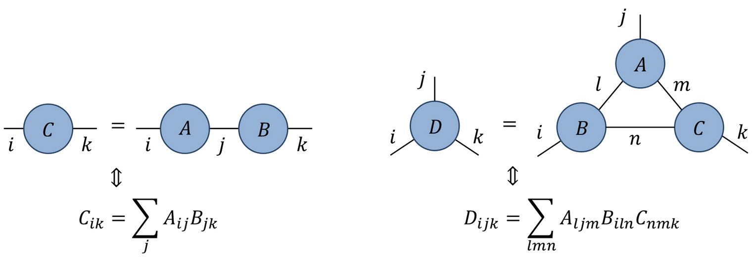
Penrose tensor notation

Graphical notation due to Roger Penrose
Rank $N$ tensor is represented as blob with $N$ legs:

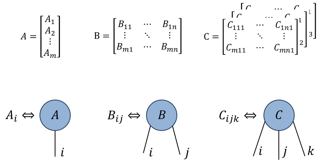
The tensor notation. Source: Glen Evenbly

Represent tensor contractions by connecting legs:

Tensor contractions. Left: matrix multiplication. Right: something more complicated

Example: ground state of spin chain

Simplest example: Heisenberg chain for spin-1/2:

\[ H = \sum_{j=1}^N \left[\sigma^x_j \sigma^x_{j+1} + \sigma^y_j \sigma^y_{j+1} + \sigma^z_j \sigma^z_{j+1} \right] \]

$\sigma^{x,y,z}$ are usual Pauli matrices and subscript $j$ means that matrix acts only the $j$th index of the wavefunction
Usually impose periodic boundary conditions: $\sigma^a_{j+N}=\sigma^a_j$

In tensor diagram notation

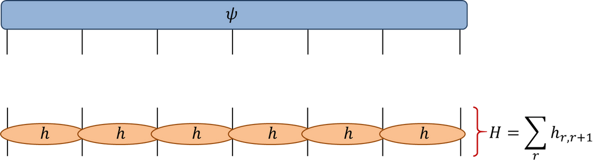
Number of components of wavefunction $\psi_{a_1,\ldots a_N}$ is $2^N$

\[ H\ket{\Psi} = E\ket{\Psi} \]

Naive matrix-vector multiplication has complexity $O(2^{2N})$: very bad idea.
Take advantage of structure, using sparsity of Hamiltonian
$H=\sum_j h_{j,j+1}$ consists of a sum of local terms, each acting on neighbouring pair

Define function that acts on wavefunction with each $h_{j,j+1}$

# by Glen Evenbly (c) for www.tensors.net, (v1.2) - last modified 6/2019

def doApplyHam(psiIn: np.ndarray,
               hloc: np.ndarray,
               N: int,
               usePBC: bool):
  """
  Applies local Hamiltonian, given as sum of nearest neighbor terms, to
  an input quantum state.
  Args:
    psiIn: vector of length d**N describing the quantum state.
    hloc: array of ndim=4 describing the nearest neighbor coupling.
    N: the number of lattice sites.
    usePBC: sets whether to include periodic boundary term.
  Returns:
    np.ndarray: state psi after application of the Hamiltonian.
  """
  d = hloc.shape[0]
  psiOut = np.zeros(psiIn.size)
  for k in range(N - 1):
    # apply local Hamiltonian terms to sites [k,k+1]
    psiOut += np.tensordot(hloc.reshape(d**2, d**2),
                           psiIn.reshape(d**k, d**2, d**(N - 2 - k)),
                           axes=[[1], [1]]).transpose(1, 0, 2).reshape(d**N)

  if usePBC:
    # apply periodic term
    psiOut += np.tensordot(hloc.reshape(d, d, d, d),
                           psiIn.reshape(d, d**(N - 2), d),
                           axes=[[2, 3], [2, 0]]
                           ).transpose(1, 2, 0).reshape(d**N)

  return psiOut

Complexity is $O(N 2^N)$
$2^N$ arises from tensor contractions over indices of a pair of sites for each assignment of the remaining $N-2$ indices
Still exponential, but exponentially better than $O(4^N)$!

Use this to instantiate a LinearOperator which is passed into eigenvalue solver (scipy.sparse.linalg.eigsh)

"""
by Glen Evenbly (c) for www.tensors.net, (v1.2) - last modified 06/2020
"""

from scipy.sparse.linalg import LinearOperator, eigsh
from timeit import default_timer as timer

# Simulation parameters
model = 'XX'  # select 'XX' model of 'ising' model
Nsites = 18  # number of lattice sites
usePBC = True  # use periodic or open boundaries
numval = 1  # number of eigenstates to compute

# Define Hamiltonian (quantum XX model)
d = 2  # local dimension
sX = np.array([[0, 1.0], [1.0, 0]])
sY = np.array([[0, -1.0j], [1.0j, 0]])
sZ = np.array([[1.0, 0], [0, -1.0]])
sI = np.array([[1.0, 0], [0, 1.0]])
if model == 'XX':
  hloc = (np.real(np.kron(sX, sX) + np.kron(sY, sY))).reshape(2, 2, 2, 2)
  EnExact = -4 / np.sin(np.pi / Nsites)  # Note: only for PBC
elif model == 'ising':
  hloc = (-np.kron(sX, sX) + 0.5 * np.kron(sZ, sI) + 0.5 * np.kron(sI, sZ)
          ).reshape(2, 2, 2, 2)
  EnExact = -2 / np.sin(np.pi / (2 * Nsites))  # Note: only for PBC


# cast the Hamiltonian 'H' as a linear operator
def doApplyHamClosed(psiIn):
  return doApplyHam(psiIn, hloc, Nsites, usePBC)


H = LinearOperator((2**Nsites, 2**Nsites), matvec=doApplyHamClosed)

# do the exact diag
start_time = timer()
Energy, psi = eigsh(H, k=numval, which='SA')
diag_time = timer() - start_time

# check with exact energy
EnErr = Energy[0] - EnExact  # should equal to zero

print('NumSites: %d, Time: %1.2f, Energy: %e, EnErr: %e' %
      (Nsites, diag_time, Energy[0], EnErr))

NumSites: 18, Time: 3.00, Energy: -2.303508e+01, EnErr: 0.000000e+00

Check out Glen Evenbly’s site is you’d like to learn more about these methods!