Floating point and ODEs

0.1  + 0.2 == 0.3

False

• What’s going on?

Integers

• Something simpler

1 + 1 == 2

True

• Integers can be represented in binary

3 == 0b11 # Ooctal `0o` or hexadecimal `0h`

True

• Binary string representation using bin function

bin(-2)

'-0b10'

• Python allows for arbitrarily large integers

• No possibility of overflow or rounding error

2**100

1267650600228229401496703205376

• Only limitation is memory!

• Numpy integers are a different story

import numpy as np
np.int64(2**100)

OverflowError: Python int too large to convert to C long

• Since NumPy is using C the types have to play nicely

• Range of integers that represented with 32 bit numpy.int32s is \(\approx\pm 2^{31} \approx \pm 2.1 × 10^9\) (one bit for sign)

• 64 bit numpy.int64s lie in range \(\approx\pm 2^{63} \approx \pm 9.2 × 10^{18}\)

• Apart from the risk of overflow when working NumPy’s integers there are no other gotchas to worry about

Floating point numbers

• \(0.1 + 0.2 \neq 0.3\) in Python is that specifying a real number exactly would involve an infinite number of bits

• Any finite representation necessarily approximate

• Representation for reals is called floating point arithmetic

• Essentially scientific notation

\[\text{significand} \times \text{exponent} \]

• Named floating point because number of digits after decimal point not fixed

• Requires choice of base, and Python’s floating point numbers use binary

• Numbers with finite binary representations behave nicely

0.125 + 0.25 == 0.375

True

• For decimal numbers to be represented exactly we’d have to use base ten. Can be achieved with decimal module:

from decimal import *
Decimal('0.1') + Decimal('0.2')

Decimal('0.3')

• But: there’s nothing to single out decimal representation in physics (as opposed to, say, finance)

• A specification for floating point numbers must give

  1. Base (or radix) \(b\)
  2. Precision \(p\), the number of digits in the significand \(c\). Thus \(0\leq c \leq b^{p}-1\).
  3. A range of exponents \(q\) specifed by \(\text{emin}\) and \(\text{emax}\) with \(\text{emin}\leq q+p-1 \leq \text{emax}\).

• With one bit \(s\) for overall sign, a number then has form \((-1)^s\times c \times b^q\).

• Smallest positive nonzero number that can be represented is \(b^{1 + \text{emin} - p}\) (corresponding to the smallest value of the exponent) and largest is \(b^{1 + \text{emax}} - 1\).

\[ (-1)^s\times c \times b^q \]

• Representation isn’t unique: (sometimes) could make significand smaller and exponent bigger

• A unique representation is fixed by choosing the exponent to be as small as possible.

• Representing numbers smaller than \(b^{\text{emin}}\) involves a loss of precision, as number of digits in significand \(<p\) and exponent takes its minimum value (subnormal numbers)

• If we stick with normal numbers and a \(p\)-bit significand, leading bit will be 1 and so can be dropped from the representation: only requires \(p-1\) bits.

• Specification for floating point numbers used by Python (and many other languages) is contained in the IEEE Standard for Floating Point Arithmetic IEEE 754

• Default Python float uses 64 bit binary64 representation (often called double precision)

• Here’s how those 64 bits are used:

  • \(p=53\) for the significand, encoded in 52 bits
  • 11 bits for the exponent
  • 1 bit for the sign

• Another common representation is 32 bit binary32 (single precision) with:

  • \(p=24\) for the significand, encoded in 23 bits
  • 8 bits for the exponent
  • 1 bit for the sign

Floating point numbers in NumPy

• NumPy’s finfo function tells all machine precision

np.finfo(np.float64)

finfo(resolution=1e-15, min=-1.7976931348623157e+308, max=1.7976931348623157e+308, dtype=float64)

• Note that \(2^{-52}=2.22\times 10^{-16}\) which accounts for resolution \(10^{-15}\)

• This can be checked by finding when a number is close enough to treated as 1.0.

x=1.0
while 1.0 + x != 1.0:
    x /= 1.01 
print(x)

1.099427563084686e-16

• For binary32 we have a resolution of \(10^{-6}\).

np.finfo(np.float32)

finfo(resolution=1e-06, min=-3.4028235e+38, max=3.4028235e+38, dtype=float32)

• Taking small differences between numbers is a potential source of rounding error

• Solution: \(x-x'=x(1-\gamma^{-1})\sim x\beta^2/2\sim 4.2\text{mm}\).

import numpy as np
from scipy.constants import c
beta = 384400e3 / (76 * 3600) / c
gamma = 1/np.sqrt(1 - beta**2)
print(1 - np.float32(1/gamma), 1 - np.float64(1/gamma))

0.0 1.0981660025777273e-11

The dreaded NaN

• As well as a floating point system, IEEE 754 defines Infinity and NaN (Not a Number)

np.array([1, -1, 0]) / 0

array([ inf, -inf,  nan])

• They behave as you might guess

2 * np.inf, 0 * np.inf, np.inf > np.nan

(inf, nan, False)

• NaNs propagate through subsequent operations

2 * np.nan

nan

• If you get a NaN somewhere in your calculation, you’ll probably end up seeing it somewhere in the output

• (this is the idea)

Differential equations with SciPy

Newton’s fundamental discovery, the one which he considered necessary to keep secret and published only in the form of an anagram, consists of the following: Data aequatione quotcunque fluentes quantitates involvente, fluxiones invenire; et vice versa. In contemporary mathematical language, this means: “It is useful to solve differential equations”.

Vladimir Arnold, Geometrical Methods in the Theory of Ordinary Differential Equations

• Solving differential equations is not possible in general

\[ \frac{dx}{dt} = f(x, t) \]

• Cannot be solved for general \(f(x,t)\)

• Formulating a system in terms of differential equations represents an important first step

• Numerical analysis of differential equations is a colossal topic in applied mathematics

• Important thing is to access existing solvers (and implement your own if necessary) and to understand their limitations

• Basic idea is to discretize equation and solution \(x_j\equiv x(t_j)\) at time points \(t_j = hj\) with some step size \(h\)

Taraji P. Henson as Katherine Johnson in Hidden Figures

Euler’s method

\[ \frac{dx}{dt} = f(x, t) \]

• Simplest approach: approximate LHS of ODE

\[ \frac{dx}{dt}\Bigg|_{t=t_j} \approx \frac{x_{j+1} - x_j}{h} \]

\[ x_{j+1} = x_j + hf(x_j, t_j) \]

\[ x_{j+1} = x_j + hf(x_j, t_j) \]

• Once initial condition \(x_0\) is specified, subsequent values obtained by iteration

\[ \frac{dx}{dt}\Bigg|_{t=t_j} \approx \frac{x_{j+1} - x_j}{h} \]

• forward finite difference: why?

• So that update rule is explicit formula for \(x_{j+1}\) in terms of \(x_j\)

• If we had used backward derivative we would end up with backward Euler method \[ x_{j+1} = x_j + hf(x_{j+1}, t_{j+1}) \] which is implicit

• This means that the update requires an additional step to numerically solve for \(x_{j+1}\)

• Although this is more costly, there are benefits to the backward method associated with stability (as we’ll see)

Truncation error

• In Euler scheme we make an \(O(h^2)\) local truncation error

• To integrate for a fixed time number of steps required is proportional to \(h^{-1}\)

• The worst case error at fixed time (the global truncation error) is \(O(h)\)

• For this reason Euler’s method is first order

• More sophisticated methods typically higher order: the SciPy function scipy.integrate.solve_ivp uses fifth order method by default

Midpoint method

• Midpoint method is a simple example of a higher order integration scheme

\[ \begin{align} k_1 &\equiv h f(x_j,t_j) \\ k_2 &\equiv h f(x_i + k_1/2, t_j + h/2) \\ x_{j+1} &= x_j + k_2 +O(h^3) \end{align} \]

• \(O(h^2)\) error cancels!

• Downside is that we have two function evaluations to perform per step, but this is often worthwhile

Rounding error

• More computer time \(\longrightarrow\) smaller \(h\) \(\longrightarrow\) better accuracy?

• This ignores machine precision \(\epsilon\)

• Rounding error is roughly \(\epsilon x_j\)

• If \(N\propto h^{-1}\) errors in successive steps treated as independent random variables, relative total rounding error will be \(\propto \sqrt{N}\epsilon=\frac{\epsilon}{\sqrt{h}}\)

• Will dominate for \(h\) small

Stability

• Euler method may be unstable, depending on equation

• Simple example:

\[ \frac{dx}{dt} = kx \]

import numpy as np
import matplotlib.pyplot as plt

def euler(h, t_max, k=1):
    """
    Solve the equation x' = k x, with x(0) = 1 using
    the Euler method. 

    Integrate from t=0 to t=t_max using stepsize h for
    num_steps = t_max / h.
    
    Returns two arrays of length num_steps: t, the time coordinate, and x_0, the position.
    """
    num_steps = int(t_max / h)
    # Allocate return arrays
    x = np.zeros(num_steps, dtype=np.float32)
    t = np.zeros(num_steps, dtype=np.float32)
    x[0] = 1.0  # Initial condition
    for i in range(num_steps - 1):
        x[i+1] = x[i] + k * x[i] * h
        t[i+1] = t[i] + h  # Time step
    return t, x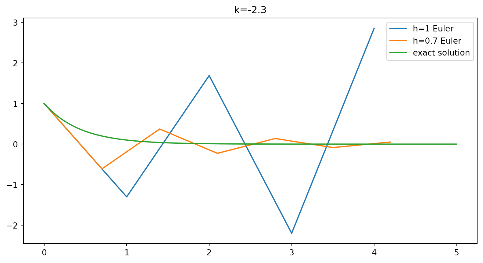

• For a linear equation Euler update is a simple rescaling

\[ x_{j+1} = x_j(1 + hk) \]

• Region of stability is \(|1 + hk|\leq 1\)

• You can check that backward Euler method eliminates the instability for \(k<0\).

Using SciPy

• Coming up with integration schemes is best left to the professionals

• Try integrate module of the SciPy library

• scipy.integrate.solve_ivp provides a versatile API

Reduction to first order system

• All these integration schemes apply to systems of first order differential equations

• Higher order equations can always be presented as a first order system

• We are often concerned with Newton’s equation

\[ m\frac{d^2 \mathbf{x}}{dt^2} = \mathbf{f}(\mathbf{x},t) \] which is three second order equations

• Turn this into a first order system by introducing the velocity \(\mathbf{v}=\dot{\mathbf{x}}\), giving six equations

\[ \begin{align} \frac{d\mathbf{x}}{dt} &= \mathbf{v}\\ m\frac{d \mathbf{v}}{dt} &= \mathbf{f}(\mathbf{x},t) \end{align} \]

• Pendulum equation

\[ \ddot \theta = -\sin\theta \] which can be cast as

\[ \begin{align} \dot\theta &= l\\ \dot l &= -\sin\theta \end{align} \]

• Solving using SciPy requires defining a function giving RHS

def pendulum(t, y): return [y[1], -np.sin(y[0])]
# The pendulum equation: y[0] is theta and y[1] is l

Then call solve_ivp

from scipy.integrate import solve_ivp
import matplotlib.pyplot as plt

t_max = 1000
pendulum_motion = solve_ivp(pendulum, [0, t_max], [2, 0], dense_output=True)

• Option dense_output=True specifies that a continuous solution should be found

• Returned object pendulum_motion has sol property that is an instance of OdeSolution. sol(t) returns the computed solution at \(t\) (this involves interpolation)

• Use this to plot pendulum’s trajectory in \(\theta- l\) phase plane, along with contours of conserved energy function

\[ E(\theta, l) = \frac{1}{2}l^2 - \cos\theta \]

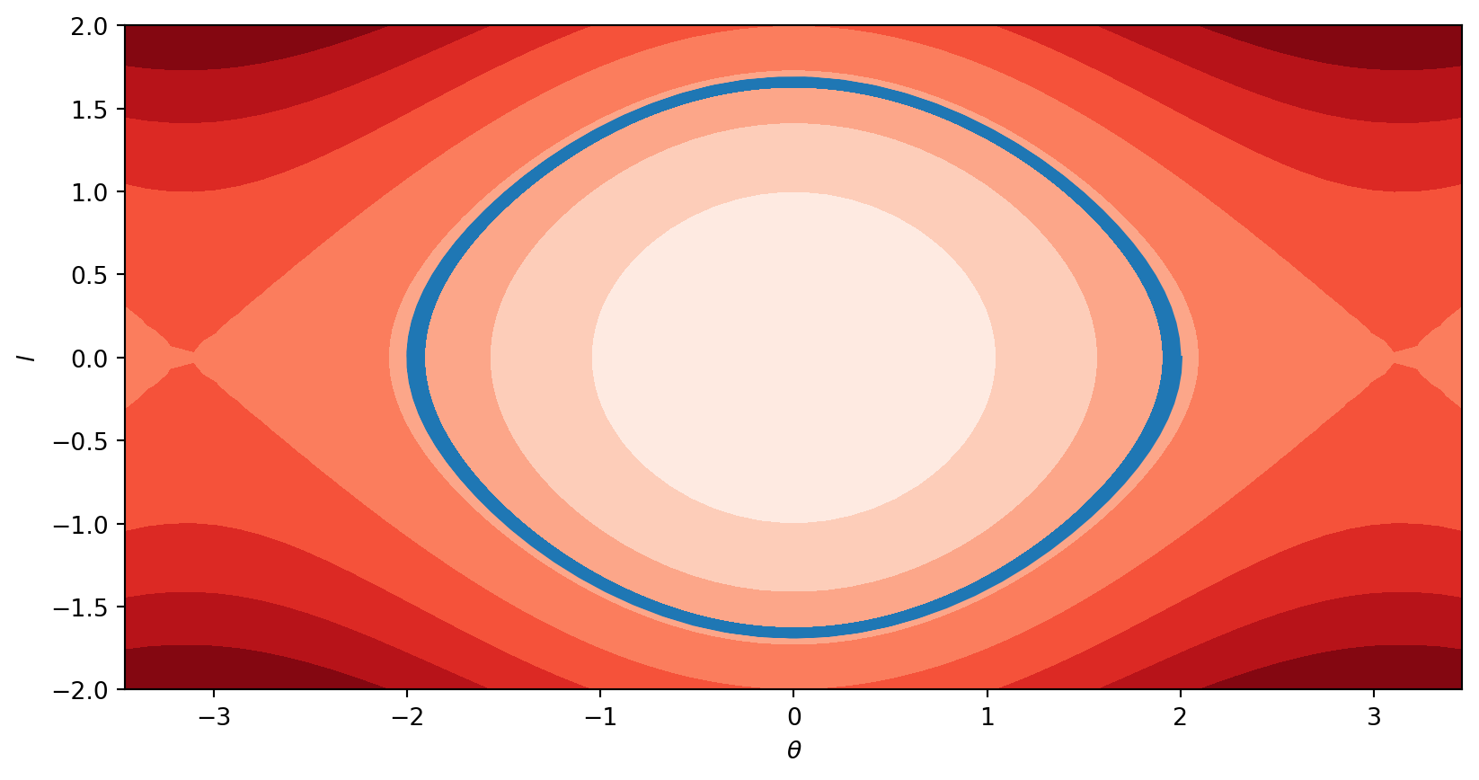
Thickness of blue line is due to variation of energy over \(t=1000\) trajectory (measured in units where the frequency of linear oscillation is \(2\pi\))

• We did not have to specify a time step

• This is determined adaptively by solver to keep estimate of local error below atol + rtol * abs(y)

• Default values of \(10^{-6}\) and \(10^{-3}\) respectively

• Monitoring conserved quantities is a good experimental method for assessing the accuracy of integration

• Alternative dense_output=True is to track “events”

• User-defined points of interest on trajectory

• Supply solve_ivp with functions event(t, x) whose zeros define the events. We can use events to take a “cross section” of higher dimensional motion

Hénon–Heiles system

• Model chaotic system with origins in stellar dynamics

\[ \begin{align} \dot x &= p_x \\ \dot p_x &= -x -2\lambda xy \\ \dot y &= p_y \\ \dot p_y &= - y -\lambda(x^2-y^2). \end{align} \]

• Example of Hamilton’s equations

• Phase space is now four dimensional and impossible to visualize.

• Conserved energy is

\[ E = \frac{1}{2}\left(p_x^2+p_y^2 + x^2 + y^2\right) + \lambda\left(x^2y-\frac{1}{3}y^3\right) \]

• \(\lambda=0\) the HH system corresponds to an isotropic 2D harmonic oscillator with conserved angular momentum

\[ J = x p_y - y p_x \]

• Take Poincaré section with \(x=0\). A system with energy \(E\) must lie within the curve defined by

\[ E = \frac{1}{2}\left(p_y^2 + y^2\right) -\frac{\lambda}{3}y^3 \]

• From \(x=0\) generate section of given \(E\) by solving for \(p_x\)

\[ p_x = \sqrt{2E-y^2-p_y^2 + \frac{2\lambda}{3}y^3} \]

def henon_heiles(t, z, 𝜆): 
    x, px, y, py = z
    return [px, -x - 2 * 𝜆 * x * y, py, -y - 𝜆 * (x**2 - y**2)]

def px(E, y, py, 𝜆):
    return np.sqrt(2 * E - y**2 - py**2 + 2 * 𝜆 * y**3 / 3)

def section(t, y, 𝜆): return y[0] # The section with x=0

t_max = 10000
𝜆 = 1
hh_motion = []
for E in [1/10, 1/8, 1/6]:
    hh_motion.append(solve_ivp(henon_heiles, [0, t_max], [0, px(E, 0.1, -0.1, 𝜆), 0.1, -0.1], events=section, args=[𝜆], atol=1e-7, rtol=1e-7))

• Plot a section of phase space with increasing energy, showing transition from regular to chaotic dynamics

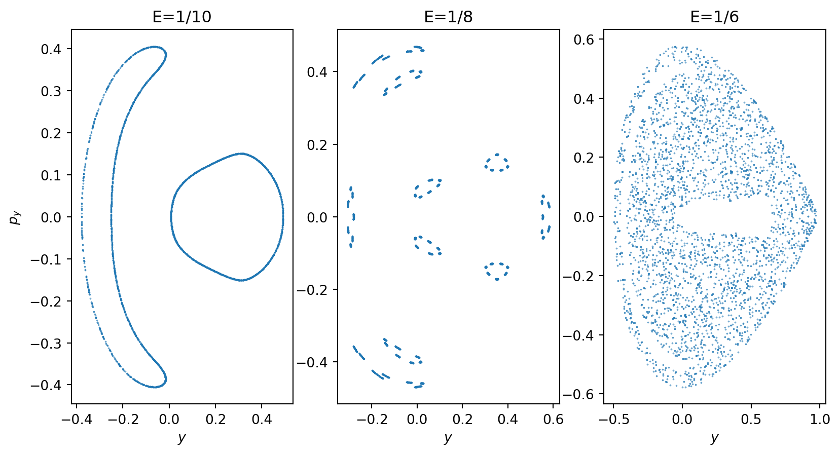
• Nice demo on Poincaré sections if you’d like to learn more